ftp://ftp.sgi.com/other/bspfaq/faq/bspfaq.html#2.txt

BSP Tree Frequently Asked Questions (FAQ)

Indexed Listing

An indexed version of this document is available for those who prefer faster loading.

---

Questions

1. CHANGES
2. ABOUT THIS DOCUMENT
3. ACKNOWLEDGEMENTS
4. HOW CAN YOU CONTRIBUTE?
5. ABOUT THE PSEUDO C++ CODE
6. WHAT IS A BSP TREE?
7. HOW DO YOU BUILD A BSP TREE?
8. HOW DO YOU PARTITION A POLYGON WITH A PLANE?
9. HOW DO YOU REMOVE HIDDEN SURFACES WITH A BSP TREE?
10. HOW DO YOU COMPUTE ANALYTIC VISIBILITY WITH A BSP TREE?
11. HOW DO YOU ACCELERATE RAY TRACING WITH A BSP TREE?
12. HOW DO YOU PERFORM BOOLEAN OPERATIONS ON POLYTOPES WITH A BSP TREE?
13. HOW DO YOU PERFORM COLLISION DETECTION WITH A BSP TREE?
14. HOW DO YOU HANDLE DYNAMIC SCENES WITH A BSP TREE?
15. HOW DO YOU COMPUTE SHADOWS WITH A BSP TREE?
16. HOW DO YOU EXTRACT CONNECTIVITY INFORMATION FROM BSP TREES?
17. HOW ARE BSP TREES USEFUL FOR ROBOT MOTION PLANNING?
18. HOW ARE BSP TREES USED IN DOOM?
19. HOW CAN YOU MAKE A BSP TREE MORE ROBUST?
20. HOW EFFICIENT IS A BSP TREE?
21. HOW CAN YOU MAKE A BSP TREE MORE EFFICIENT?
22. HOW CAN YOU AVOID RECURSION?
23. WHAT IS THE HISTORY OF BSP TREES?
24. WHERE CAN YOU FIND SAMPLE CODE AND RELATED ONLINE RESOURCES?
25. REFERENCES

http://research.microsoft.com/en-us/um/people/hoppe/pm.pdf

progressive mesh.pdf

http://www.gamasutra.com/view/feature/3177/subdivision_surface_theory.php

At Siggraph '98, Pixar unveiled a short animated film. Christened Geri’s Game, it was, to quote its Academy Award press release, the “endearing tale of an aging codger who likes to play chess in the park against himself.” Not only was it artistically stunning, but it was also a technological powerhouse. The short served as a vehicle to demonstrate Pixar’s latest addition to its production environment, a surface scheme known as subdivision surfaces.

Subdivision surfaces are a way to describe a surface using a polygonal model. Like the polygonal model, the surface can be of any shape or size — it’s not limited to a rectangular patch. Unlike that polygonal model, the surface itself is perfectly smooth. Subdivision surface schemes allow you to take the original polygonal model and produce an approximation of the surface by adding vertices and subdividing existing polygons. The approximation can be as coarse or as detailed as your needs allow. Because Pixar’s rendering system requires everything to be broken into polygons that are a half-pixel across, subdivision surfaces allowed them to tessellate automatically to that level everywhere. As such, the artists didn’t need to worry about how close Geri was to the camera. While your game probably can’t quite deal with half-pixel polygons, whatever size you do choose, your models can scale up and down in polygon count with the speed of the machine and their distance from the camera.

Along with Pixar’s work, quite a few researchers are actively tackling issues in the area of subdivision surfaces, and several Siggraph papers each year advance them academically and put them to use in solving problems. By now, they are a fairly mature technology, and a compelling contender among scalability solutions.The technology itself is, for the most part, not new, but its application up until recently has been fairly limited. Indeed, Geri’s Game is still one of the only compelling demonstrations of subdivision surfaces. Nonetheless, it brought attention to subdivision surfaces as a relatively new, up-and-coming technique for implementing scalable geometry.

The game development community realizes that scalable geometry techniques are an important part of developing next-generation game engines. The spread between high-end and low-end hardware seems to get bigger each year (thanks to current and forthcoming geometry accelerators such as Nvidia’s GeForce 256 and S3’s Savage2000), forcing game developers to find ways to cater to the masses that use low-end machines while building in features that make the most of hardcore gamers’ advanced hardware. As a result, on the low end our engines should still be capable of using fewer than 10,000 polygons per scene, but on the high end, the sky’s the limit: even hundreds of thousands of polygons per scene can cruise along at 60 frames per second. Scalable geometry techniques such as subdivision surfaces are therefore necessary to accommodate this variation in hardware capabilities.

In this article, a number of different kinds of subdivision surfaces will be discussed. As a preliminary warning, this article is entirely theory. Next month, we’ll look at an example implementation of one of the schemes, the modified butterfly, which I’ll discuss here. Keep in mind as you read this article that not every concept described here will be practical for use in your engine. Indeed, some subdivision surface models may not be feasible for use in games at all. But knowing the strengths and weaknesses of the various models will help you make the right decision for your next game.

The What and the Why

First, what is a subdivision surface? The obvious answer is that it’s a surface generated through subdivision. To elaborate, every subdivision surface starts with an original polygonal surface, called a control net. Then the surface is subdivided into additional polygons and all the vertices are moved according to some set of rules. The rules for moving the vertices are different from scheme to scheme, and it is these rules that determine the properties of the surface. The rules of most schemes (including all the ones discussed here) involve keeping the old vertices around, optionally moving them, and introducing new vertices. There are schemes that remove the old vertices at each step, but they’re in the definite minority.

The one thing the control net and the eventual surface (called the limit surface) have in common is that they are topologically the same. Topology is a way of describing the structure of a surface that isn’t changed by an elastic deformation, that is, a stretching or twisting. A good example and common joke is that to a topologist, a coffee cup and a donut are identical. The donut hole corresponds to the hole in the handle of the coffee mug. On the other hand, a sphere and coffee mug are not topologically equivalent, since no amount of stretching and twisting can punch a hole in that sphere.

Topology is one reason that subdivision surfaces are worth a look. With Bézier or B-spline patches, modeling complex surfaces amounts to trying to cover them with pieces of rectangular cloth. It’s not easy, and often not possible if you don’t make some of the patch edges degenerate (yielding triangular patches). Furthermore, trying to animate that object can make continuity very difficult, and if you’re not very careful, your model will show creases and artifacts near patch seams.

That’s where subdivision surfaces come in. You can make a subdivision surface out of any arbitrary (preferably closed) mesh, which means that subdivision surfaces can consist of arbitrary topology. On top of that, since the mesh produces a single surface, you can animate the control net without worrying about seams or other continuity issues.

As far as actual uses in games, I believe that subdivision surfaces are an ideal solution for character modeling. Environments and other parts of a game generally don’t have the fine detail or strange topology that would require subdivision surfaces, but characters can have joint areas that are particularly hard to model with patches, and characters are in constant animation, which makes maintaining continuity conditions very important.

The basics. Before we start discussing individual schemes, let’s look at the basic characteristics of subdivision surfaces in general. This gives us a framework for classifying and comparing the schemes as we come across them. Most of these characteristics carry notable implications with them, whether they are implied computational costs or implied ease-of-use considerations, or anything else. These will usually be the criteria on which you might choose one scheme above another.

Continuity: the holy grail. The first characteristic of a scheme is its continuity. Schemes are referred to as having Cⁿ continuity, where n determines how many derivatives are continuous. So if a surface is C⁰ continuous, it means that no derivatives are continuous, that the surface itself doesn’t have open holes. If a surface is C¹ continuous, it means that the surface is closed and that its tangents are continuous (so there aren’t any sharp seams).

This probably won’t be a major selling point of one scheme above another, since just about every scheme has C¹ continuity everywhere. Some have C² continuity in some places, but the majority have areas where the best they can claim is C¹. So most schemes are alike in this regard.

However, continuity is most certainly worth mentioning because it’s one of the major reasons to think about using subdivision surfaces in the first place. After all, Pixar could have modeled Geri using as many polygons as they wanted, since they’re not running their movies in real time. But no matter how many polygons they used, you could get close enough that Geri’s skin would look faceted from the polygons. The point of using a subdivision model is that you have that ideal limit surface at which you can always throw more and more polygons as you get closer and closer to, no matter how high the display resolution or how close the model is to the screen. Only a very small portion of the real world is flat with sharp edges. For everything else, there’s subdivision surfaces.

To Interpolate or not to Interpolate...

While the degree of continuity is generally the same for all subdivision schemes, there are a number of characteristics that vary notably between schemes. One important aspect of a scheme is whether it is an approximating scheme or an interpolating scheme. If it’s an approximating scheme, it means that the vertices of the control net don’t lie on the surface itself. So, at each step of subdivision, the existing vertices in the control net are moved closer to the limit surface. The benefit of an approximating scheme is that the resulting surface tends to be very fair, having few undulations and ripples. Even if the control net is of very high frequency with sharp points, the scheme will tend to smooth it out, as the sharpest points move the furthest onto the limit surface. On the other hand, this can be to the approximating scheme’s detriment, too. It can be difficult to work with, as it’s harder to envision the end result while building a control net, and it may be hard to craft more undulating, rippling surfaces as the scheme fights to smooth them out.

Figure 1. Two schemes subdivide a  tetrahedron. The left scheme is  approximating, and the right is interpolating.

If it’s an interpolating scheme, it means that the vertices of the control net actually lie on the limit surface. This means that at each recursive step, the existing vertices of the control net are not moved. The benefit of this is that it can be much more obvious from a control net what the limit surface will look like, since the control net vertices are all on the surface. However, it can sometimes be deceptively difficult to get an interpolating surface to look just the way you want, as the surface can develop unsightly bulges in areas where it strains to interpolate the vertices and still maintain its continuity. Nonetheless, this is usually not a tremendous problem.

Figure 1 shows examples of an approximating scheme (on the left) and an interpolating scheme (on the right). The white outline is the control net, and the red wireframe is the resulting surface after a few subdivision steps. You can see the difference quite clearly: the approximating surface seems to pull away from the net, while the interpolating surface flows through the vertices of the net.

Surfaces in Uniform

Another set of characteristics of a scheme brings in four more terms. A scheme can be either uniform or nonuniform, and it can be either stationary or nonstationary. These terms describe how the rules of the scheme are applied to the surface. If the scheme is uniform, it means that all areas of a control net are subdivided using the same set of rules, whereas a nonuniform scheme might subdivide one edge one way and another edge another way. If a scheme is stationary, it means that the same set of rules is used to subdivide the net at each step. A nonstationary scheme, on the other hand, might first subdivide the net one way, and then the next time around use a different set of rules.

All the schemes we’ll talk about here are fundamentally both uniform and stationary. There are some extensions to these schemes that make them nonstationary or nonuniform, but there aren’t many subdivision schemes that are fundamentally nonstationary or nonuniform. One of the main reasons for this is that most of the mathematical tools we have for analyzing schemes are unable to deal with dynamically changing rules sets.

Subdivision Shape

Another characteristic of a scheme, albeit less significant than the prior ones, is whether it is triangular or quadrilateral. As the names would imply, a triangular scheme operates on triangular control nets, and a quadrilateral scheme operates on quadrilateral nets. Clearly, it would be inconvenient if you had to restrict yourself to these primitives when building models. Therefore, most quadrilateral schemes (including the one discussed here) have rules for subdividing n-sided polygons. For triangular schemes, you generally need to split the polygons into triangles before handing them over to be subdivided. This is easy enough to do, but one downside is that for some schemes, the way you break your polygons into triangles can change the limit surface. The changes are usually minor, though, so you simply need to be consistent: if you randomly choose which diagonal of a quadrilateral to split on every frame, you’ll end up with popping artifacts.

Figure 2 shows examples of a triangular subdivision scheme as compared to a quadrilateral scheme. Notice that the triangular scheme only adds new vertices along the edges, whereas the quadrilateral scheme needs to add a vertex in the center of each face. This is one reason why triangular schemes tend to be somewhat easier to understand: their rules have that one fewer step in them.

Figure 2. The differences between the tessellation used by a triangular scheme (top) and a quadrilateral scheme (bottom).

Extraordinary Vertices

The preferred vertex valence is another property of subdivision schemes. The valence of a vertex is the number of edges coming out of it. Most every vertex a scheme produces during subdivision has the same valence. Vertices of that valence are the regular vertices of a scheme. Vertices of any other valence are known as extraordinary vertices. Their effect depends on the subdivision scheme, but historically there have been problems analyzing the limit surface near extraordinary vertices. As we look at various schemes, we’ll see the effect that extraordinary vertices have on each one.

Most schemes don’t ever produce extraordinary vertices during subdivision, so the number of extraordinary vertices is set by the original control net and never changes. Figure 3 is an example of two steps of a triangular scheme with an extraordinary vertex in the center. Notice how it remains the only extraordinary vertex after a step of subdivision. Also note that the valence of the regular vertices is 6. This is common for triangular schemes, as they all tend to split the triangles in the same way — by adding new vertices along the edges and breaking each triangle into four smaller triangles.

Figure 3. A triangular net (left) and after one subdivision step (right). The red vertex is extraordinary.

Surface Evaluation

Surface evaluation is the process of taking a control net, adding vertices, and breaking faces into more, smaller faces to find a better polygonal approximation of the limit surface. There are a number of ways to evaluate a subdivision surface. All subdivision schemes can be evaluated recursively. Furthermore, most (including all the ones discussed here) can be explicitly evaluated at the vertex points of the control net. For interpolating schemes, this means that you can explicitly calculate the surface normals at the vertices using what are called tangent masks. For approximating schemes it means you can also explicitly calculate the vertex’s limit position, using what are called evaluation masks. In this context, a mask isn’t the same kind of mask that you might use during binary arithmetic. Our masks are more analogous to the masks worn at a masquerade. They are like stencil cutouts, shapes that can be “placed” on the control net, and their shape determines which of the surrounding vertices are taken into account (and how much effect each has) in determining the end result, be it the vertex location or its tangent vectors. Figure 4 shows a visual example of applying a mask to a surface at a vertex.

Figure 4. A hypothetical mask. Here, the white region is a mask used to dictate which vertices are used in a computation involving the  red vertex.

An important aspect of evaluation is the scheme’s support. The support refers to the size of the region considered during evaluation. A scheme is said to have compact support if it doesn’t have to look very far from the evaluation point. Compact support is generally desirable because it means that changes to a surface are local — they don’t affect the surface farther away.

A Note on Notation

Since the original authors of many subdivision schemes weren’t operating in concert with one another, the notation used between schemes tends to vary fairly wildly. Here, I’ve tried to stick with a fairly consistent notation. When talking about a specific vertex, it is v. If it matters what level of recursion it’s at, that level i is indicated as a superscript, so the vertex is vⁱ. The vertex’s valence is N. The neighboring vertices of the vertex are e_j where j is in the range [0,N–1]. Again, if the level of recursion matters, that level i is a superscript, so eⁱ_j is the jth edge vertex at level i. I try to use this notation everywhere, but there are a few places where it’s much clearer to use a different notation.

The one problem with a standard notation is that if you access some of the references at the end of this article, they will very likely use their own, different notation. As long as the concepts make sense, though, it shouldn’t be difficult to figure out someone else’s naming convention.

The Polyhedral Scheme

The polyhedral scheme is about the simplest subdivision scheme of all, which makes it a good didactic tool but not the kind of scheme you’d ever actually want to use. It’s a triangular scheme where you subdivide by adding new vertices along the midpoints of each edge, and then break each existing triangle into four triangles using the new edge vertices. A simple example is shown in Figure 5. The problem with this, of course, is that it doesn’t produce smooth surfaces. It doesn’t even change the shape of the control net at all. But it serves to demonstrate some concepts fairly well.

Figure 5. Two steps of subdividing a  triangle with the polyhedral scheme.

The scheme is clearly interpolating since it doesn’t move the vertices once they’re created. It’s also triangular, since it operates on a triangular mesh. Furthermore, the scheme is uniform since the edge’s location doesn’t affect the rules used to subdivide it, and stationary since the same midpoint subdivision is used over and over. The surface is only C0 continuous, since along the edges of polygons it doesn’t have a well-defined tangent plane. The regular vertices of this scheme are of valence 6, as that’s the valence of new vertices created by the scheme. However, this scheme is simple enough that it doesn’t suffer because of its extraordinary vertices.

The evaluation of the scheme isn’t hard at all. You can evaluate it recursively using the subdivision rules. As far as evaluation and tangent masks go, it’s clear that we don’t need an evaluation mask, since the points are already on the limit surface. Tangent masks don’t really make any sense, since our surface isn’t smooth and therefore doesn’t have well-defined tangents everywhere.

Figure 6 shows a tetrahedron control net in white with a red wireframe of the surface after a few subdivision steps of the polyhedral scheme.

Figure 6. A tetrahedron  control net (in white) and  a polygonal surface approximation (in red) produced using the  polyhedral scheme.

http://misofruit.co.kr/seojewoo/programming/project2312.htm

지형 처리 방법

3D게임의 가장 큰 특징은 가상의 공간을 자유롭게 돌아다닐 수 있다는 데서 찾을 수 있다. 따라서 대개 3D 게임은 
굉장히 큰 공간을 배경으로 진행되는 경우가 많다. 그런데, 공간이 커지면 커질수록 동시에 처리해야 하는 데이터의
양도 급증해 컴퓨터가 감당할 수 없을 정도의 부하를 주게 된다. 이러한 이유로 3D게임에는 효율적인 공간 처리방법
들이 연구되고 구현돼 왔지만, 모든 경우를 자유롭게 처리할 수 있는 이상적인 방법은 없고 제작하려는 게임에 가장
적절한 방법을 선택해 구현하는 것이 현명하다. 여기서 소개하는 방법은 가장 널리 사용되고 있으며 효율도 우수하
지만 사전 작업의 시간을 많이 필요로 하므로 정적인 지형의 경우에 알맞다.

BSP

BSP는 Binary Space Partition의 약자로, 말 그대로 이분적인 공간 분할 방법을 의미한다. 큰 지형을 이진트리 형태
호 분석해 노드 정보를 구성하고 이를 참조해 대상 물체를 찾아내는 것이 BSP의 기본 원리로, 유명한 돔에서 사용한
이후로 널리 알려졌다. BSP는 간단하게 다음과 같은 과정으로 실시된다.

(1)모델에 존재하는 면 중 하나를 선택한다. 만약 선택할 면이 없으면 종료한다.

(2)선택한 면의 위에 겹치는 모습의 무한 평면을 상상해 이것으로 공간을 분할한다. 이 때 무한 평면에 걸치는 면이
    있으면 이것은 두 개로 잘라진다.(이미 처리된 면은 생략).

(3)선택한 면의 법선 방향을 앞으로, 반대방향을 뒤로 해서 앞쪽에 있는 면들에 대해 (1)의 과정을 제귀적으로 수행
    한다.

(4)선택한 면의 뒤쪽에 있는 면들에 대해 (1)의 과정을 재귀적으로 수행한다. 이 과정을 실제의 예를 들어 설명해보
    겠다.

<그림 8 >과 같은 지형이 있고, 이것을 BSP를 이용해 <그림9 >처럼 분할해보자.
우선 임의의 한면을 선택한다. 여기서는 10면을 선택한다. 그러면 이것은 최상위 노드에 위치하고, 이 평면을 중심
으로 앞뒤로 분할하게 된다. 면의 앞쪽에 있는 면들은 왼쪽 노드에 속하고, 뒤쪽은 오른쪽 노드가 된다.
이때 분단면이 관통하는 5면은 분할돼 각각 5a/5b로 나눠진다. 이제 분할된 면을 기준으로 (1)의 과정을 반복한다.

이번에는 3면을 선택해 수행한다. 이때 주의할점은 이미 처리된 면이나 부모 노드가 다른 쪽은 대상에서 제외된다는
것이다. 우선 앞 노드에 대해 앞의 과정을 재귀적으로 계속 처리하고 완료하면 다시 최상위의 뒤쪽 노드에 대해서도
같은 식으로 적용한다. 그러면 <그림 10>과 같이 BSP노드 정보가 완성된다.

마지막에 위치한 노드는 최종적으로 존재할 수 있는 노드로서 이 노드의 안쪽에 있으면 지형 내에 존재하는것으로
판단된다. NULL노드에 위치하거나 최종 노드의 바깥쪽에 있으면 지형을 벗어나는 것으로 간주한다. 이제 이러한 
정보를 갖고 임의의 위치나 지형 안에 포함되는지를 검사해보자.

<그림 12 >처럼 별표의 위치에 게임의 캐릭터가 존재한다고 가정할 때 BSP노드의 정보를 따라 검색하면, 우선 지
정된 위치는 10면의 뒤쪽 -> 6면의 뒤쪽 -> 9a면의 앞쪽 -> 5b면의 앞쪽이라는 방식으로 도형안에 속해 있음을 알
수 있다. BSP트리 생성의 과정을 C++로 작성하면 다음과 같다.

BspNode * BSP :: Make(Model * pModel )
      //노드 생성
      BspNode *pNode = new BSP_Node( );
      //모델에서 분단면으로 쓸 폴리곤 선택
      Polygon *pPolygon = pModel- >GetPartitionPolygon();
      //더이상 분할할 수 없는 경우
      if ( pPolygon ==NULL ) return node;

      //분단면을 트리 구조에 보존
      pNode -> SetPartitionPlane ( pPolygon );
      //선택한 면으로 모델을 이등분
      Model *pFront, *pBack ;
      pFront = SplitFrontModel (pModel, pPolygon);
      pBack = SplitBackModel (pModel, pPolygon);

      //BSP 트리를 만들기 위해 재귀적으로 분할해 트리에 추가
      pNode->LinkToFront ( Make ( pFront ) );
      pNode->LinkToBack ( Make ( pBack) );

이러한 방식으로 BSP를 이용하면 복잡한 지형도 검사 대상을 획기적으로 줄여 짧은 시간 내에 처리할 수 있고,깊이
정렬이 자동적으로 이뤄져 렌더링 속도가 빨라지는 효과도 누릴 수 있다.

http://talkon.egloos.com/1222472

dPVS 상용로 판매되는 라이브러리 같다. 동작 방법은 버퍼에 씬정보를 가지고 있으면서 오브잭트가 그려질지 안그려질지를 결정하면서 컬링이 이루어 지는 방식이고 순서는 다음과 같다.

1. Occlusion Buffer를 만든다. (frame, zbuffer or stencil)

2. View Frustum으로 Object를 컬링한다.

3. 컬링되고 남은 오브잭트는 가까운 것에서 먼 곳 순으로 정렬해준다.

4. 그려야할 오브잭트가 버퍼와 비교해 렌더링 하고 갱신한다.

기본적인 개념은 위와 같이 진행된다.

으음... 

http://www.gpgstudy.com/forum/viewtopic.php?p=9888

Hierarchical Occlusion Map (HOM) 란 놈도 있는데 이 놈은 어떨지...

http://www.misofruit.co.kr/seojewoo/programming/project23111.htm

PVS(Potentially visible set)은 visible surface determination(보이는 면 결정)알고리즘의 하나이다. 공간상에서 폴리곤들은 다른 폴리곤에 가려서 보이지 않는 경우가 많다. 그래서 보이는 폴리곤들만을 결정해서 렌더링한다는 이론이다. 퀘이크엔진의 경우, 지형을 leaf라고 하는 여러 개의 영역으로 나눈 뒤(leaf를 방이라고 생각하면 이해가 쉬울 것이다.) 각 영역에서 보일 수 있는 영역들의 리스트(potentially visible set: PVS)를 미리 계산하여서 Lookup 테이블에 저장해 둔다. 게임 동작중에는 카메라의 위치에 따라 해당 위치의 leaf에서 보이는 영역에 대한 리스트를 Lookup테이블을 참조하여서 얻을 수 있다. 그리고 이 영역들만을 렌더링하게 되고 나머지 leaf들은 렌더링에 포함되지 않는다.

감자님의 사이트에 올려져 있는 글입니다.
http://www.gamza.net/ez2000/ezboard.exe?db=Algorithm&action=list&page=0 

** Portal을 이용한 PVS작성개념 **
copyrightⓒ 김성수 [2001년 02월 21일]

퀘이크가 '보이는 공간 작성'에 사용하는 방법은? 포탈 입니다. 
포탈은 두개의 공간과 연결되어있고, 공간은 여러개의 포탈과 연결될수 있죠. 
퀘이크가 하는짓은...궤이크 유틸소스/Vis/flow.c 의 void RecursiveLeafFlow (...) 만 분석해보시면 됩니다. 
개념을 잡기위해 간단하게 그림을 몇장 그려봤습니다.

공간 A에서 보이는 공간리스트를 작성하기 위한 그림입니다.
우선 공간A의 임의의 포탈Pab와 그와 연결된 공간 B의 Pab가 아닌 임의의 포탈Pbc를 잡습니다.
Pbc와 연결된 또다른 공간을 C라하고 Pab위에서 Pbc를 통해 보이는 C의 포탈을 찾습니다.
이때 일부만 보이는 포탈은 클리핑을 합니다.

                 ::::::::::::::::::::::::::::::::::::::::::::::::::::::::::::::::::::::::::::::::::::::::::::::::::::::::::::::::::::::::::::::

다음은 마소 2001년 9월호에 올라와 있는 글이다.

일어라 구글 번역..

http://www.kotaku.jp/2013/01/cry_engine_mine_craft.html

'마인 크래프트' (영상)

참고)

http://en.wikipedia.org/wiki/Convex_hull

요렇게 stage에 무작위로 찍은 점들이 있다치자.

원기둥 쯤으로 생각하고 원기둥들을 실로 감싸면 아래 그림처럼 될 것이다. 가운데쯤 있는 원기둥은 강력접착제로 붙이지 않고는 차례가 돌아가지 않을 것이다.

위 원기둥이 그저 눈에 보이라고 그려 놓은 것이고 크기가 없는 점이라고 하면 다음과 같이 될 것이다.

오목한 부분이 없는 폴리곤 형태다. 그래서convex hull이라 부르는게 아닐까 싶다.

기하알고리즘들이 그렇듯 눈으로 보면 대충 알겠는데 이걸 코드로 바꾸려면… 어렵다.

Convex hull관련 알고리즘도 굉장히 여러가지가 있고 그럭저럭 쉽게 이해한 Graham Scan 방식을 설명해보려한다.

1. 첫 시작점을 어떤걸로 정할지
2. 둘러칠 점의 순서는 또 어떻게 정할지
3. 요 점이 내부에 포함될 점인지 아니면 외곽에 해당하는 점이지는 어떻게 알아낼지

3가지가 핵심이다.

GrahamScan은 시작점과 다른 모든 점이 이루는 각도를 가지고 가장 작은 각에서 가장 큰 각을 순서로 선을 잇는다.

시작점은 가장 상하좌우 가장 끝에 있는 걸 고른다.

이렇게 얻은 각도를 로 양의 정수로 고쳐서 소팅하거나 (Math.atan2의 경우 마이너스 값이 나올 수도 있다.)

양의 각도, 음의각도 두개를 따로 소팅한 뒤 합치는 것도 방법일 수 있겠다.

플래시에서는 맨 좌측에 있으면서 가장 위에 있는 녀석을 고르는 것이 각도 구할 때 유리할 것이다. 음의 각도가 나오지 않는다.

선을 이어나가는 방향은 ccw나 cw 한방향을 만족시켜야 되는데... 무슨 말인가 하면:

1번그림처럼 시계방향으로 회전한 다음 시계반대방향으로 회전하게 되면 오목한 부분이 생긴다는 말이다.

2번에서 시계반대방향이 생긴경우 해당 점을 제외시킨다.

3번 그림처럼 다음 점과 방향검사를 한다. 처음 시도한 방향과 같으면 선을 연결한다.

이러한 방향은 두 벡터의 외적으로 쉽게 알 수 있다. 외적의 값이 0이면 collinear(공선벡터: 스칼라 값은 다르더라도 방향이 같다)이고 음수이면 왼쪽(cw:시계방향)으로 돌고 양수이면 오른쪽(ccw:반시계방향)으로 돈다.

그럼 시작점을 찾아보자.

시작점과의 각도를 구한다. (시작점이 원점이 되도록 한다.)

http://blog.naver.com/helloktk/80050600334

주어진  convexhull (counterclockwise)에 임의로 한 점을 추가하여 새로운 convexhull 를 구성하는 procedure 다. 작동의 원리는 아래의 그림과 같다. 만약에 주어진 점이  convexhull 의 내부점이면 원래의 convexhull이 반환된다.

std::vector<CPoint>
chull_point_merge(CPoint Q, std::vector<CPoint>& chull) {
    std::vector<CPoint> out;

    int n = chull.size();

    if(n < 2) {
        out = chull; out.push_back(Q);
        return  out;
    }

    bool pushed = false;

    bool prev = isright(chull[n-1], chull[0], Q)  ; 
    for(int i = 0; i < n; i++) {
        bool curr = isright(chull[i], chull[(i+1)%n], Q)  ;
        if(prev) {
            if(curr) {
                if(!pushed) {
                    out.push_back(Q);
                    pushed = true;
                }
                continue;
            }
            else if(!pushed) {
                out.push_back(Q);
                pushed = true;
            }
        }
        out.push_back(chull[i]);
        prev = curr;
    } 
    return out;
}

//C is on the right side of segment AB ;
bool isright(CPoint A, CPoint B, CPoint C) {
    B -= A; 
    C -= A;
    return (B.x * C.y - B.y * C.x) < 0   ;
}

[밀리언 파티클 시스템]

http://210.96.133.182/knowledge/trend/abroad/__icsFiles/afieldfile/2010/05/02/72218.pdf

[파티클 엔진]

http://www4.wittenberg.edu/academics/mathcomp/computer_science/students/student_projects/computer%20graphics/bixler_guthikonda/index.html

[파티클시스템]

http://www.google.co.kr/url?sa=t&rct=j&q=%ED%8C%8C%ED%8B%B0%ED%81%B4%EC%8B%9C%EC%8A%A4%ED%85%9C&source=web&cd=1&ved=0CDQQFjAA&url=http%3A%2F%2Fcfs7.tistory.com%2Fupload_control%2Fdownload.blog%3Ffhandle%3DYmxvZzIwOTc5NEBmczcudGlzdG9yeS5jb206L2F0dGFjaC8wLzEyLnBkZg%3D%3D%26filename%3DClass08.pdf&ei=0c4wT5OHKIueiAfFvIyABQ&usg=AFQjCNHAP0WEevj95zn1t2ZjOwNtkONxUg&sig2=a1O1RjcbZHWnNqlwe-3qVQ&cad=rjt

GPU를 이용한 실시간 분수 시뮬레이션을 위한 파티클 시스템

http://visualcomputing.yonsei.ac.kr/papers/domestic/KCC08_sh.pdf

ppt 인데 소스 좀 있는것

http://graphics.pcu.ac.kr/nicesk/DirectX_2/10week/14Particle.pdf

http://www.google.co.kr/url?sa=t&rct=j&q=%ED%8C%8C%ED%8B%B0%ED%81%B4%EC%8B%9C%EC%8A%A4%ED%85%9C&source=web&cd=65&ved=0CEAQFjAEODw&url=http%3A%2F%2Fdis.dankook.ac.kr%2Flectures%2Fgame07%2Fattachment%2F1363750330.pdf&ei=ztYwT72WLaOkiAeft8SVBQ&usg=AFQjCNFFetFktZ4v9UFLaxLaDlxJevXHsA&sig2=bFSOrdtnlJTuSDCppIEvig&cad=rjt

http://blog.naver.com/doridori3510/30130730459

water reflection 수면 반사 방법! DirectX 2011/12/15 10:12 http://blog.naver.com/doridori3510/30126259858

http://blog.naver.com/doridori3510/30127128770

+ 수면 아래 장면 만들기

수면 위의 반사장면 만드는것과 동일하게 물을 기준으로 아래 장면을 텍스쳐로 만든후.

물 평면에 투영한다 !

좀더 좋은 효과를 만들기위해서 물과 지형과의 거리에 비례해서 알파값을 계산한다 !

+ 프레넬 공식에 비례해서 수면 위 장면, 수면 아래 장면을 섞어서 그릴지 계산.

+ 범프 텍스쳐를 기준으로, 수면 위, 아래 장면의 UV를 흔든다.

+ 범프 텍스쳐를 노멀벡터로 생각해서 각각의 조명을 계산한다.

범프 텍스쳐를 기준으로 노멀 벡터를 구하는데, 노멀벡터의 Y값을 세우기 위해서 Z값을 Y값으로 생각해서 채워 넣는다.

이 방법이 통하는것은.

물이 평면이고 접선공간으로 변환해서 하는 결과값 ( bump.rgb * 조명방향[접선공간] ) = (bump.rbg)

이 성립하기 때문이다.

정확하게 말하자면, bump에서 읽어온 노멀값과 접선공간으로 변환된 조명과 연산해야한다.

// 조명의 방향을 접선공간으로 변형.
o.LightDir.x = dot(worldLightDirection, T);
o.LightDir.y = dot(worldLightDirection, B);
o.LightDir.z = dot(worldLightDirection, N);

// ViewVec 역시 접선공간으로 변형.

float3 viewVec = normalize(vWorldCameraPos - worldPos);
o.ViewVec.x = dot(viewVec, T);
o.ViewVec.y = dot(viewVec, B);
o.ViewVec.z = dot(viewVec, N);

+ 최종적인 물의 칼라값 결정

원래 물 고유의 색상과 혼합한다.

< 최종적인 스샷 >

세부적인 수치같은거 조절해야하는데... 귀찮다 ㅋㅋㅋㅋㅋㅋㅋㅋㅋㅋㅋㅋㅋ

암튼 색상이랑 수치 비율이랑 조절하면 더 예뻐질것임. 성형수술같네;ㅁ;

비행기는 계속해서 움직이고 수면에 실시간으로 반사함 !

< 수치 조절 좀 했더니 >엉? 사진올려놓고 보니 비슷비슷한가?ㅋㅋ 실제로 보면 아닌데 ㅜ.ㅜ

구글링하다 찾은 펄린노이즈

알려진 펄린노이즈의 방법은 전체적인 대강의 윤곽은 비슷 할 수 있찌만 내부적으로 세세히 조금씩 다른

방법들이 있는데 아래 필자가 쓴 방법이 좀더 빠른 연산을 보인다고 한다

tip : 일부 내적에 대한 부족한 설명을 '편집' 이라는 부분에 보충 설명을 해놓음

1차로 예를 들면..

펄린노이즈는 각 정수 단위 사이에들어오는 성분(x) 에 대해서 -1 ~1 사이의 난수 값을 생성해 낸다

각 구간마다 난수벡터를 만들어 놓고 성분(x) x 가 어느 정수 구간 1 거리 사이안에 들어 간다면

ex( 244 ~255) 이 구간 244 와 255 에 설정되어 있는 난수값과 244 와 255 에서 x 값을 향하는 벡터와의 각 내적 값들을

3차 방정식이 x 축이 되는 x ----- > 3차 --------> 선형 보간----------- > v0 ~ v1 의 값으로 보간 되는

즉 일반적으로 선형 보간 된 값이 v0 또는 v1 쪽으로 더 쏠리는 보간값의 형태가 되어

최종 결과 값은 v0 와 v1 의 중간 값보다는 v0 쪽이나 v1 쪽에 더 영향을 받는 난수 값을 얻게 된다

2차는 1차 사이의 보간을 통해

3차는 2차 사이의 보간을 통해 구한다

http://webstaff.itn.liu.se/~stegu/TNM022-2005/perlinnoiselinks/perlin-noise-math-faq.html#toc-algorithm

The Perlin noise math FAQ

by Matt Zucker

v. 1.0, last updated February 2001

Table of Contents

• About this document
  
• What is Perlin noise?
  
• How do you generate Perlin noise?
  
• Computational complexity
  
• Speeding it up
  
• Looping noise
  
• Seamlessly tiling noise
  

About this document

So far, I have found two really great sources for information about Perlin noise. They are Ken Perlin's Making Noise web site, which has a comprehensive introduction to the topic, and Hugo Elias's page, which features some algorithms and a few more detailed examples of applications. This document is intended to complement those two valuable resources by explaining in more depth, hopefully in plain English, some of the math involved in Ken Perlin's original implementation of Perlin noise.

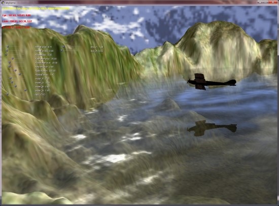
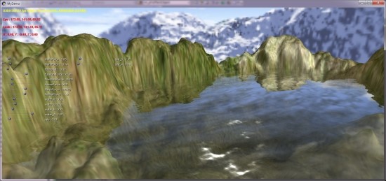
I wrote a demo program in C++ that includes a Perlin noise texture class, which I hope provides a decent example of C++ code for Perlin noise. You can find the demo at http://www.robo-murito.net/code.html.

If I've made any grave errors or you just want to comment, feel free to email me.

What is Perlin noise?

Perlin noise is function for generating coherent noise over a space. Coherent noise means that for any two points in the space, the value of the noise function changes smoothly as you move from one point to the other -- that is, there are no discontinuities.

Non-coherent noise (left) and Perlin noise (right)

When I talk about a noise function, I mean a function that takes a coordinate in some space and maps it to a real number between -1 and 1. Note that you can make noise functions for any arbitrary dimension. The noise functions above are 2-dimensional, but you can graph a 1-dimensional noise function just like you would graph any old function of one variable, or consider noise functions returning a real number for every point in a 3D space.

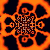
These images were all created using nothing but Perlin noise:

Besides these trivial images, there are countless interesting applications for noise in computer graphics. Look at Hugo Elias' page or Ken Perlin's pages for some pretty examples, in-depth explanations and nifty ideas.

How do you generate Perlin noise?

I've seen implementations on the internet that take non-coherent noise, as shown above, and smooth it (with something like a blur function) so it becomes coherent noise, but that can end up being more computationally expensive than the function I'll present here, which is more or less theoriginal implementation that Ken Perlin came up with. The problem with Perlin's implementation on its own was that that reading the descriptions of the math published on Perlin's website was a bit like reading Greek -- it took me about a week of reading his code and notes to figure out the actual geometric interpretations of the math. So hopefully this document can trim down that learning curve.

Let's look at the 2D case, where we have the function

noise2d(x, y) = z,

with x, y, and z all real (floating-point) numbers. We'll define the noise function on a regular grid, where grid points are defined for each whole number, and any number with a fractional part (i.e. 3.14) lies between grid points. Consider finding the value of noise2d(x, y), with x and y both notwhole numbers -- that is, the point (x, y) lies somewhere in the middle of a square in our grid. The first thing we do is look at the gridpointssurrounding (x, y). In the 2D plane, we have 4 of them, which we will call (x₀, y₀), (x₀, y₁), (x₁, y₀), and (x₁, y₁).

The 4 grid points bounding (x, y)

Now we need a function

g(x_grid, y_grid) = (g_x, g_y)

which takes each grid point and assigns it a pseudorandom gradient of length 1 in R² ('gradient' is just the name for an ordered pair or vector that we think of as pointing in a particular direction). By pseudorandom, we mean that g has the appearance of randomness, but with the important consideration that it always returns the same gradient for the same grid point, every time it's calculated. It's also important that every direction hasan equal chance of being picked.

The 4 pseudorandom gradients associated with the grid points

Also, for each grid point, we generate a vector going from the grid point to (x, y), which is easily calculated by subtracting the grid point from (x, y).

Vectors from the grid points to (x, y)

Now we have enough to start calculating the value of the noise function at (x, y). What we'll do is calculate the influence of each pseudorandom gradient on the final output, and generate our output as a weighted average of those influences.

First of all, the influence of each gradient can be calculated by performing a dot product of the gradient and the vector going from its associated grid point to (x, y). A refresher on the dot product -- remember, it's just the sum of the products of all the components of two vectors, as in

(a, b) · (c, d) = ac + bd .

Since I'm really tired of writing subscripts, we'll just refer to these 4 values as s, t, u, and v, where

s = g(x₀, y₀) · ((x, y) - (x₀, y₀)) ,
t = g(x₁, y₀) · ((x, y) - (x₁, y₀)) ,
u = g(x₀, y₁) · ((x, y) - (x₀, y₁)) ,
v = g(x₁, y₁) · ((x, y) - (x₁, y₁)) .

So here's a 3D-ish picture of some influences s, t, u, and v coming out of the R² plane (note that these probably wouldn't be the actual values generated by the dot products of the vectors pictured above).

Influences from the grid points

Geometrically, the dot product is proportional to the cosine of the angle between two vectors

, though its unclear to me

------------------------------------------------------------------------------------------

편집 : 다른 곳에서 보니....

내적이 의미 하는게 사각 셀(사각형 안의 x,y 에 해당하는) 것의 4 귀퉁위의 각 높이값을

말하는 듯..

------------------------------------------------------------------------------------------

if that geometrical interpretation helps one visualize what's going on. The important thing to know at this point is that we have four numbers, s, t, u, and v which are uniquely determined by (x, y) and the pseudorandom gradient function g. Now we need a way to combine them to get noise2d(x, y), and as I suggested before, some sort of average will do the trick.

I'm going to state the obvious here and say that if we want to take an average of four numbers, what we can actually do is this:

1. find the average of the first pair of numbers
2. find the average of the second pair of numbers
3. average those two new numbers together

-- and that's the strategy we'll take here. We'll average the "front" values s and t first, then average the "rear" values u and v. This works to our advantage because the points below s and t, and similarly below u and v vary only in the x dimension -- so we only have to worry about dealing with one dimension at a time.

We're not taking a plain vanilla-flavored average here, but instead, a weighted average. That is, the value of the noise function should be influenced more by s than t when x is closer to x₀ than x₁ (as is the case in the pictures above). In fact, it ends up being nice to arrange things so that x and y values behave as if they are slightly closer to one grid point or the other than they actually are because that has a smoothing effect on the final output. I know that sounds really silly, but noise without this property looks really stupid. In fact, it sounds so silly that I'm going to write it again: we're going to want the input point to behave as if its closer to one grid point or another than it actually is.

This is where we introduce the concept of the ease curve. The function 3p² - 2p³ generates a nice S-shaped curve that has a few characteristics that are good for our purposes.

Meet the ease curve

What the ease curve does is to exaggerate the proximity its input to zero or one. For inputs that are sort of close to zero, it outputs a numberreally close to zero. For inputs close to one, it outputs a number really close to one. And when the input is exactly one half, it outputs exactly one half. Also, it's symmetrical in the sense that it exaggerates to the same degree on both sides of p = ½. So if we can treat one grid point as the zero value, and the other as the one value, the ease curve has the exact smoothing effect that just we said we wanted.

Ok, I've droned on long enough, it's calculation time: first, we take the value of the ease curve at x - x₀ to get a weight S_x. Then we can find the weighted average of s and t by constructing a linear function that maps 0 to s and 1 to t, and evaluating it at our x dimension weight S_x. We'll call this average a. We'll do the same for u and v, and call the result b.

Finding the first two averages using linear interpolation

The above figures should satisfy you that no matter where x happens to fall in the grid, the final averages will always be between s and t, and u andv, respectively. Mathematically, this is all simple to calculate:

S_x = 3(x - x₀)² - 2(x - x₀)³
a = s + S_x(t - s)
b = u + S_x(v - u)

Now we find our y dimension weight, S_y, by evaluating the ease curve at y - y₀, and finally we take a weighted sum of a and b to get our final output value z.

A weighted sum of the first two averages yields the final output

And there you have it. So all you have to do is call the noise function for every pixel you want to color, and you're done. Probably.

An interesting consequence of all of this is that the noise function becomes zero when x and y are both whole numbers. This is because the vector (x, y) - (x₀, y₀) will be the zero vector. Then the dot product of that vector and g(x₀, y₀)will evaluate to zero, and the weights for the averages will also always be zero, so that the zero dot product will influence the final answer 100%. The funny thing is that looking at the noise function, you would never guess that it ends up being zero at regular intervals.

Computational complexity

If you want to extend the noise function to n dimensions, you'll need to consider 2ⁿ grid points, and perform 2^{(n - 1)} weighted sums. The implementation presented here has a computational complexity of O(2^{(n - 1)}), which means that you'll really start to drag if you want to look at 5-, 6-, or greater dimensional noises.

Speeding it up

We could increase the speed of the noise function if we didn't have to compute the pseudorandom gradient every time we called the noise function (because for every x between some x₀ and x₁ and y between some y₀ and y₁, we have to recalculate the same four gradients every time the noise function is called!) The nice thing to do would be to precalculate the gradient for every possible (x_grid, y_grid), but x_grid and y_grid are allowed to vary all over the real plane! How could we possible precalculate every value?

The neat thing about noise is that it's locally variable, but globally flat -- so if we zoom out to a large degree, it will just look like a uniform value (zero in fact). So, we don't care if the noise function starts to repeat after large intervals, because once you're zoomed out far enough to see the repeat, it all looks totally flat anyways.

So now we should feel justified in doing a little trick with modulus. Say we're doing noise in 3D, and we want to find the gradient for some grid point (i, j, k). Let's precompute a permutation table P, that maps every integer from 0 to 255 to another integer in the same range (possibly even the same number). Also, let's precompute a table of 256 pseudorandom gradients and put it in G, so that G[n] is some 3-element gradient.

Now,

g(i, j, k) = G[ ( i + P[ (j + P[k]) mod 256 ] ) mod 256 ]

But on a computer, modulus with 256 is the same thing as a bitwise and with 255, which is a very fast operation to perform. Now we've reduced the problem of a possibly involved function call into nothing but some table lookups and bitwise operations. Granted, the gradients repeat every 256 units in each dimenstion, but as demonstrated, it doesn't matter.

This speedup is also mentioned on Perlin's web page, and is actually used in his original implementation.

Looping noise

What if you want to use procedural noise to calculate a repeating animation of a licking flame or rolling clouds? It is true that noise on it's own doesn't tend to repeat discernably, and that's great for generating ever-changing images; however, if you want to prerender an animation, you'll probably want it to repeat. Given that F is your function that generates a real number from a point in noise-space, and you want your animation to repeat every t units, you define a new function that loops when z is between 0 and t:

F_loop(x, y, z) = ( (t - z) * F(x, y, z) + (z) * F(x, y, z - t) ) / (t)

Now each function call takes twice as long to calculate, but since you're probably not going to use this cycling technique in real time, it probably doesn't matter.

The explanation

Consider the graph of a noise function F(x, y, z) for some fixed x and y. The problem is, you want F(0) = F(t) and there is no guarantee that will be the case with any old x, y, and t. Actually, since any given x and y should have no influence on the repeating aspect of the animation, we can for all practical purposes throw them out while we're developing our repeating function, and consider the simplified case of a one-dimensional noise function F(z).

A one-dimensional noise function

We need to take this function and change it into one where it is guaranteed that F(0) = F(t). Here's an expanded view of our noise function showing its behavior from -t to t:

The same, function, ranging over a positive and negative domain

Now we define a new function F'(z) that behaves like F(z) when z is near zero, but behaves like F(z - t) when z is near t. If you think about it, you see that F'(0) = F(0), and that F'(t) = F(t - t) = F(0). We can do this with a simple linear interpolation by considering a linear function which is equal to F(z) at 0, and equal to F(z - t) at t.

High school algebra tells us that this linear function has a slope of

(rise) / (run) = (F(z - t) - F(z)) / (t - 0) = (F(z - t) - F(z)) / t

and an intercept of F(z). Now we set up F' as this linear interpolation operating on z:

F'(z) = slope(z) + intercept
= ( (F(z - t) - F(z)) / t )(z) + F(z)
= ( ( (z) * F(z - t) - (z) * F(z) ) / t ) + F(z)
= ( ( (z) * F(z - t) - (z) * F(z) ) / t ) + (t / t) * F(z)
= ( (z) * F(z - t) - (z) * F(z) + (t) * F(z)) / (t)
= ( (z) * F(z - t) + (t-z) * F(z) ) / (t)
= ( (t-z) * F(z) + (z) * F(z - t) ) / (t)

Which is basically the same as the function given above. If you look at F' next to F, you can see that the function does indeed repeat in that F'(0) = F'(t). Also notice that the peaks just to the right of F'(0) are the same as the peaks just to the right of F'(0), and that the peaks just to the left ofF'(t) are virtually identical to the peaks just to the left of F(0).

The old function (left), and the new, repeating function (right)

If you had a little calculus and too much free time, you could prove that this looping (and the tiling in the next section) is truly seamless: not only does F(0) = F'(t), but all their derivatives should match up as well. Which means that no one should be able to tell where the repeat actually happens.

Seamlessly tiling noise

Say you're using a noise function to generate textures for a polygon-based engine. Chances are, you might want the textures to be tileable. You can extend the above example to generate tileable 2-dimensional noise that repeats every w units in the x dimension and every h units in the y dimension. This will require a weighted sum of four calls to the original function (which again, for lack of imagination, we will call F).

F_tileable(x, y) = (
F(x, y) * (w - x) * (h - y) +
F(x - w, y) * (x) * (h - y) +
F(x - w, y - h) * (x) * (y) +
F(x, y - h) * (w - x) * (y)
) / (wh)

A pattern should be emerging here, so it shouldn't surprise you that you'll need evaluate a weighted sum of 8 calls to the noise function if you want to have a repeating animation that tiles in the x and y dimenstions. I'm not going to write it out here out of space considerations, and also because it should be evident what the sum will be.

http://apophysis.org/

Apophysis Freeware fractal flame editor for Windows Apophysis Forum Apophysis at SourceForge Home Downloads Tutorials Links

---

http://www.ultrafractal.com/download/index.php

• 

Download your copy of Ultra Fractal 5 here:

Windows

Mac OS X

Download Ultra Fractal for Windows

Version 5.04 — Windows 7, Vista and XP

After installing, Ultra Fractal will run as a free trial version for 30 days. If you already have purchased a license key, simply enter it when Ultra Fractal starts to unlock full functionality.

Installation (Windows)

After downloading, double-click on the downloaded file to install Ultra Fractal. When you first start Ultra Fractal, a welcome screen will appear that provides access to tutorials and online help to help you to get started quickly.

Evaluation

The downloaded evaluation version is fully functional, except that exported and rendered images are marked as written by an evaluation copy. If you have a license for Ultra Fractal 5, enter it when starting the program to turn the trial version into a full version.

If you want to keep using Ultra Fractal after the 30-day trial period, you must purchase a copy in the Ultra Fractal shop. You can also purchase a site license if you need more than one copy.

See Also

Purchase

Support

Español

Deutsch

Ultra Fractal 5.04

Released August 11, 2010, version 5.04 contains bug fixes and improvements.

Release notes

Other downloads

PDF manual

Public formulas

Previous versions

The included help file is also available in PDF format for easy printing.

Download PDF manual

All rights reserved. Copyright © 1997-2012 Frederik Slijkerman