http://cafe.naver.com/ckgirl/90
| [게임프로그래머를 위한 기초 수학과 물리]제4장 벡터연산 [완성] |
1. 벡터 vs 스칼라
우리가 흔히 하는 셈에서 다루는 값은 스칼라입니다. 그냥 스칼라는 그런수죠. 우리가 초,중,고 다니면서 수학시간에 열심히 계산할때 사용한 대부분의 수. 즉 방향이 없는 크기들입니다..
벡터는 방향과 크기를 모두 함께 가지고 있는 값입니다. 내가 가고자 하는 목적지가 지금 위치로부터 100미터 떨어져 있다와 북쪽으로 100미터 떨어져있다가 스칼라와 백터의 차이점입니다.
거리나 속력은 스칼라값을 말하는 단위입니다. 변위나 속도는 벡터값을 말하는 단위이고요.
변위는 거리라는 스칼라값을 벡터로 표현한것이고 속도는 속력이라는 스칼라값을 벡터로 표현한 것입니다.
시속 100km 는 속력이고 동쪽으로 시속 100km 라고 하면 속도가 되는 것이죠.
벡터의 값에는 방향이 있는데 이것을 다루는 방법을 이야기 하자면 1차원에서는 방향이 2개 입니다. 음수나 양수로 방향을 표시할 수 있습니다. 예를 들어서 오른쪽에서 왼쪽으로 스크롤되는 횡스크롤 게임(D&D같은)이 있다고 할때 캐릭터가 오른쪽으로 가면 양수이고 왼쪽으로 가면 음수가 되는 것입니다.
마찬가지로 위에서 아래로 종스크롤되는 게임(1945 striker 같은)에서는 위로가면 양수 아래로 가면 음수가 됩니다.
실제 수를 넣어서 문제를 보자면 위아래로만 움직일 수 있는 퐁 게임에서 반사판의 중심이 (20,400)에서 (20,50)까지 움직였다면 변위는 얼마일까요?
위,아래로만 움직일 수 있기 때문에 x좌표의 값은 변화없이 20으로 고정이 됩니다. 그렇다면 y 값을 살펴볼까요. y의 값이 400 에서 50으로 달라졌네요. 따라서 변위는 -350 입니다.
변위를 다룰때는 방향을 고려하는 것이 매우 중요합니다. 스칼라 양인 거리와 벡터량인 변위는 매우 큰 차이가 있기 때문입니다. 변위를 계산할때 고려해야 할 것은 시작점과 끝점의 위치뿐이고 그 사이에 일어나는 일은 그다지 중요하지 않습니다.
풋볼경기를 예로 들어보면 다음과 같습니다.
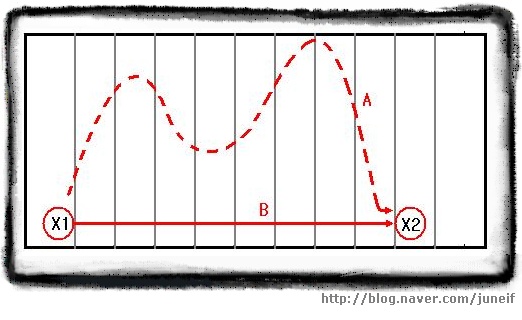 [풋볼 선수의 변위]
 볼 경기에서 한 선수가 20야드 라인에서 공을 잡고 달리기 시작합니다. 도중에 수비수들을 피해 요리조리 빠져나가며 계속 달려나가다가 50 야드 라인에서 태클을 당했다면 이 선수의 전진 거리로 인정되는건 A라인이 아니라 B 라인이 됩니다. 벡터도 이와 마찬가지입니다. 도중에 지그재그로 가던지 곧바로 가던지 결국 중요한것은 출발점과 도착점 뿐이라는 것이죠.
위의 그림에서 A 값은 스칼라 값이고 B 값은 벡터 값이 되는 것입니다.
=================================================
| 변위
| ΔX = X2 - X2
=================================================
자자 그럼 문제 나갑니다. 슈퍼마리오 게임을 하고 있는데 수평위치 200픽셀에서 시작햇습니다. 오른쪽으로 마구마구 이동하다가 250픽셀쯤 왔을때 버섯을 놓친 것을 깨닫고 다시 100픽셀에 있는 버섯을 먹고 왔습니다. 그 후 마리오는 다시 데이지 공주가있는 450 픽셀까지 달려가 공주를 만났다면 이 마리오의 최종 변위는 몇일까요? 또 실제 이동거리는 얼마일까요?
최종변위부터 계산할까요? 시작점이 200픽셀이고 도착점이 450픽셀이니 450 - 200 = 250 간단하죠?
실제 이동거리도 간단합니다. 처음 200픽셀에서 250픽셀까지 갔을때 50픽셀을 이동했고 다시 버섯이 있는 100픽셀까지 이동했으니 150 픽셀을 더 가서 현재까지 200픽셀을 이동했습니다. 그 후에 공주가 있는 450픽셀까지 이동했으니 추가로 350 픽셀을 더 이동했네요. 그래서 실제 이동거리는 550픽셀이 되는 것입니다.
2. 벡터의 기술 방법
앞에서 우리는 1차원 벡터의 방향을 기술할때 양수와 음수만으로 충분하다는 것을 알았습니다.
하지만 2차원과 3차원에서는 이것만으로는 충분하지 않습니다.
2차원에서 벡터를 기술하는 방법은 2가지가 있습니다. 그것은 바로 극좌표와 데카르트 좌표계입니다. 먼저 극좌표계부터 살펴보겠습니다.
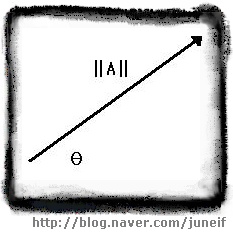 [극좌표로 표현한 벡터 A]
극좌표는 벡터가 실제로 어떤 모양인지를 파악하는 가장 쉬운 방법입니다.
===================================================================
| 벡터 A 의 크기를 ||A|| 라 하고, 벡터의 방향을 θ라 할때
| 벡터 A = ||A|| @ θ
===================================================================
데카르트 좌표는 조금 덜 직관적이지만, 벡터를 코딩할때 사용하는 형식입니다.
극좌표와 같이 길이와 방향으로 벡터를 기술하는 대신, 벡터를 수평과 수직 변위로 나타낼 수도 있으며 이것은 데카르트 좌표계의 방식과 매우 유사합니다. 데카르트 좌표를 구성하는 두가지 요소는 수평과 수직성분이며 이렇게 표현한 형식을 i j 형식이라고 합니다.
====================================================================
| 데카르트 좌표 (벡터 성분)
| 벡터의 x 축 방향의 단위벡터를 i^ , y 축 방향의 단위벡터를 j^ 라고하면,
| 벡터 B = b1 i^ + b2 j^
======================================================================
** 단위벡터를 나타내는 문자가 원래는 i 위에 ^ 이 모자처럼 씌어진 그림입니다만 키보드에서 적절한 문자를 찾을 수 없어서 뒤에다가 썻으니 이점을 숙지하여 다른 책이나 자료를 볼때 혼동하지 마시길바랍니다. 아래 그림을 참고하시기 바랍니다.
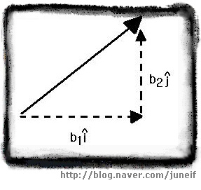
[데카르트 좌표로 표현된 벡터 B]
컴퓨터의 화면은 격자 형태로 설정되습니다. 그렇기 때문에 코딩을 할때 데카르트 좌표를 사용합니다.
혹 극좌표를 사용하려고 한다고 해도 결국은 데카르트 좌표로 변환하여 사용해야 합니다. 극좌표에서 데카르트좌표로 변환하는 방법은 아래 그림과 같습니다.
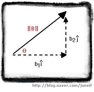 [극좌표에서 데카르트 좌표로의 변환]
 =====================================================
| 극좌표에서 데카르트 좌표로의 변환
| 벡터 A 가 ||A|| @ θ 일때
| A = b1 i^ + b2 j^
| 단, b1 = ||A|| cos θ , b2 = ||A|| sin θ
=====================================================
그럼 예문을 하나 보면서 확실히 기억해볼까요?
벡터 A가 변위 벡터이고, A = 20m @ 30˚ 일때 이 벡터를 데카르트 좌표 형식으로 변환해 보세요.
위의 공식을 잘 보세용 먼저 A를 두 요소로 분해하기 위해 사인과 코사인을 사용합니다.
b1 = || A || cos θ = 20 cos 30˚ = 20(0.8660) = 17.32
b2 = || A || sin θ = 20 sin 30˚ = 20(0.5) = 10
그래서 A = 17.32 i^ + 10 j^ 입니다.
반대로 데카르트 좌표를 극좌표로 변환도 가능합니다.
========================================================
| 벡터 B 가 b1 i^ + b2 j^ 일 때,
| ||B|| = √(b1)² + (b2)² , θ = tan-1 (b2 / b1) <--- tan-1 이 아크탄젠트라는거 알고 계시죠? ^^;;
========================================================
예제를 하나 살펴볼께요.
벡터 3i^ + 4j^ 를 극좌표로 변화하여 보세요.
먼저 B 의 크기를 계산합니다
||B|| = √(b1)² + (b2)² = √ 3² + 4² = √ 9 +16 = √25 = 5
B의 크기를 구한 다음에는 방향을 계산합니다.
θ = tan-1 ( b2 / b1 ) = tan-1 (4/3) = 53.1˚ (근사값입니다.)
따라서, 극좌표로는 B = 5 @ 53.1˚ 입니다.
데카르트 좌표를 2차원에서 3차원으로 확장 할 수도 있습니다. 2차원에는 없는 z 축을 추가해주기만 하면 됩니다. 간단하죠? 공식은 다음과 같습니다.
====================================================================================
| 3차원 데카르트 좌표 ( 벡터 성분 )
| 벡터의 x 축 방향의 단위벡터를 i^ , y축 방향의 단위벡터를 j^ , z 축 방향의 단위벡터를 k^ 라고 하면,
| 벡터 B = b1 i^ + b2 j^ + b3 k^
=====================================================================================
데카르트 좌표 형식의 벡터는 i, j 형식 대신 종종 행렬의 한 열이나 한 행으로 표기 되기도 합니다.
5
예를 들어보면 2차원 벡터 A = 5 i^ + 6 j^ 는 [5,6] 또는 [ 6 ] 으로 표기할 수 있습니다.
7
마찬가지로 3차원 벡터 B = 7 i^ + 8 j^ + 9 k^ 는 [ 7, 8 ,9 ] 또는 [ 8 ] 라고 표기할 수 있습니다.
9
3 벡터의 합과 차
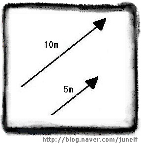
벡터량을 시각적으로 구성할 때는, 각 벡터에 화살표를 사용하는 것이 일반적입니다. 화살의 길이는 벡터의 크기를 나타내고, 화살표의 끝이 가리키는 방향이 벡터의 방향을 나타냅니다. 화살은 비례에 맞도록 그려야 하기 때문에 모든 벡터가 같은 비례를 가지도록 그리는 것이 중요합니다. 아래의 그림처럼 크기가 5m 인 벡터는 크기가 10m 인 벡터의 절반에 해당하는 길이를 가지게 됩니다.
 [화살 표로 표현한 두 벡터] 벡터를 화살표로 표시할 때, 화살표의 촉 부분을 끝점이라고 하고 그 반대쪽을 시작점이라고 부릅니다.
벡터는 어느 한점에 고정된것이 아니기 때문에 화살표의 길이와 방향만 같다면 어디든지 이동이 가능합니다. 아래의 그림처럼 끝점이 같은 두 벡터 A 와 B에서 벡터 B의 끝점을 벡터 A의 시작점으로 옮기는 것도 가능합니다.
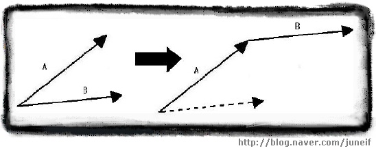 [벡터 A의 끝점과 벡터 B의 시작점을 일치하록 옮긴 벡터의 그림]
두 벡터의 시작점과 끝점을 일치하도록 만들었다면, 움직이지 않은 벡터의 시작점과 움직인 벡터의 끝점을 연결하여 새로운 벡터를 그리면 이 새 벡터가 바로 두 벡터의 합입니다.
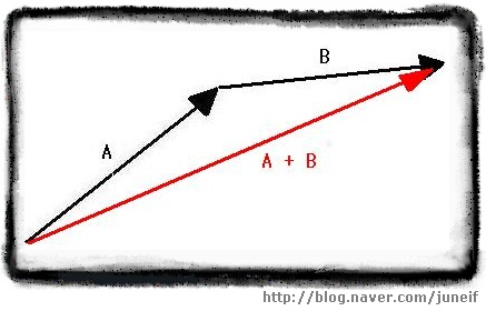 [ 벡터 A 와 벡터 B 의 합 ]
 이렇게 벡터의 합을 구할때 둘중 어떤 벡터를 옮기더라도 새롭게 만들어지는 합의 벡터는 언제나 같습니다.
즉 벡터의 합에는 교환법칙이 성립한다는 이야기가 되는 것이죠.
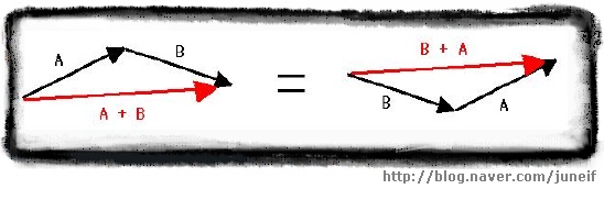 [ A + B = B + A ]
 =============================================
| 벡터 합의 교환법칙
| 임의의 벡터 A, B 에 대하여,
| A + B = B + A
=============================================
위의 그림에서 각각의 벡터 A 가 5m 라고 가정하고 벡터 B가 6m 라고 가정할때 A+B 의 벡터의 길이는 어떤가요? A=5 이고 B=6 이니 A+B =11 이라고 생각하기 쉽지만 그림을 잘 보시면 새롭게 만들어진 붉은 벡터가 기존의 두개의 검은 벡터를 더한것보다 짧게 보이죠? 이 것은 벡터의 방향이 고려되었기 때운입니다.
결국 방향이 같지 않다면 || A+B || ≠ ||A|| + ||B|| 라는 말이 됩니다.
그래서 극 좌표로 표현된 벡터는 같은 방향이 아닌이상 항상 데카르트 좌표로 변환하여 더해야 합니다.
두 벡터가 데카르트 좌표로 표현되었다면, 같은 성분의 벡터끼리 더하기만 하면 됩니다.
다시말해서 두개의 i^ 와 두개의 j^를 더하는 것이죠.
=================================================================
| 두 벡터의 합 계산
| 두 벡터 A = a1 i^ + a2 j ^ , B = b1 i^ + b2 j^ 에 대하여,
| A + B = ( a1 + b1 ) i^ + (a2 + b2) j^
=================================================================
역시 예제를 살펴보면서 확실히 이해해 봅시다.
두 벡터 C = 8i^ + 3j^ , D = 5i^ + 12j^ 에 대하여, C+D를 구하세요.
먼저 이 두 벡터를 그린후에 D의 시작점을 C의 끝점으로 옮깁니다. 거듭 강조하지만 벡터를 옮기는 과정에서 길이와 방향이 변하지 않도록 주의해 주세요.
C 의 시작점과 D의 끝점을 이어서 새로운 벡터 C + D 를 그려줍니다. 그림은 아래와 같습니다.
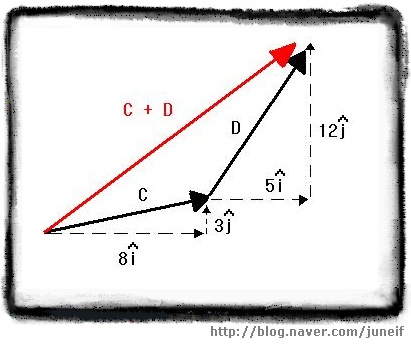 [ 벡터 C + D ]
 C + D 를 계산하는 방법은 x축 방향으로의 총 이동량과 y축 방향으로의 총 이동량을 계산하는 것입니다. 즉 두개의 i^와 두개의 j^ 를 각각 성분별로 더하는 것이죠. 이 경우에는, 다음과 같이 계산할 수 있습니다.
C + D = (8+5) i^ + (3+12) j^ = 13 i^ + 15 j^
벡터의 합을 구하는 이같은 방법은 3차원에서도 그대로 적용됩니다. 마찬가지로 3차원에서의 벡터의 합을 계산하려면 벡터는 반드시 데카르트 좌표 형식이어야 합니다.
=============================================================================
| 3차원 벡터의 합 계산
| 두 벡터 A = a1 i^ + a2 j^ + a3 k^, B = b1 i^ + b2 j^ + b3 k^ 에 대하여,
| A + B = (a1+b1) i^ + (a2+b2) j^ + (a3+b3) k^
=============================================================================
지금까지 보아온 벡터의 합과 같은 방법으로 두 벡터의 차도 구할 수 있습니다. 각 성분의 합을 구한것처럼 각 성분의 차를 구하면 됩니다. 2차원과 3차원에서의 벡터의 차 공식 나갑니다!!!!!!!!]
=================================================================
| 두 벡터 사이의 차 계산
| 두 벡터 A = a1 i^ + a2 j ^ , B = b1 i^ + b2 j^ 에 대하여,
| A - B = ( a1 - b1 ) i^ + (a2 - b2) j^
=================================================================
=============================================================================
| 3차원 벡터의 차 계산
| 두 벡터 A = a1 i^ + a2 j^ + a3 k^, B = b1 i^ + b2 j^ + b3 k^ 에 대하여,
| A - B = (a1-b1) i^ + (a2-b2) j^ + (a3-b3) k^
=============================================================================
4. 벡터의 스칼라 곱
우리들은 지금까지 공부하면서 수많은 종류의 곱셈을 해왔습니다. 양수끼리의 곱셈, 음수와 양수의 곱셈, 정수와 소수와 곱셈 등등등....... 이들 곱셈은 모두 스칼라값과 스칼라값 사이의 곱셈이었습니다. 이제 위에서 배운 백터를 써먹을 때가 됬네요. 바로 벡터와 스칼라의 곱셈을 할 차례입니다!!!!
벡터에 스칼라를 곱한다는 것은 벡터의 크기를 늘리거나 줄이는 결과를 가져옵니다. 곱하는 스칼라가 1보다 크다면 벡터는 커지고, 스칼라가 1보다 작다면 벡터의 크기는 작아집니다.
============================================================================
| 극좌표 형식 벡터의 스칼라 곱
| 임의의 벡터 A = c ||A|| @ θ 에 대하여,
| cA = c ||A|| @ θ
============================================================================
예제를 하나 살펴볼까요?
벡터 A = 3ft @ 22˚ 일때 5A 를 구하세요.
위의 공식에 바로 대입해 볼께요.
5A = 5(3ft) @ 22˚ = 15ft @ 22˚
벡터가 극좌표의 형식이 아닌 데카르트좌표 형식으로 되어 있어도 극좌표로 변환하지 않고 스칼라 곱을 구할 수 있는 방법이 있습니다. 각 성분별로 스칼라를 곱하기만 하면 됩니다. 공식은 아래와 같습니다.
=============================================================================
| 데카르트 형식 벡터의 스칼라 곱
| 임의의 스칼라 c와 임의의 벡터 A = a1 i^ + a2 j^ 에 대하여,
| cA = ca1 i^ + ca2 j^
=============================================================================
예제 고고싱~~~!!!
벡터 A = 12 i^ + 4 j^ 일때, 1/2A 를 구하세요.
바로 공식에 대입합니다.
1/2A = 1/2(12 i^) + 1/2(4 j^) = 6 i^ + 2 j^
프로그래밍에서는 정규화(normalization)라는 용어를 종종 쓰이곤 합니다. 이 용어는 벡터의 크기를 1로 맞추는 것을 뜻합니다. 벡터의 정규화는 벡터의 크기보다는 벡터의 방향만을 필요로 할 때 이용됩니다. B = i^ + j^ 에서 i^는 x 축의 양의 방향을, j^ 는 y축의 양의 방향을 가리키는 크기가 1인 벡터입니다.
벡터의 정규화는 벡터가 극좌표 형식일때는 매우 간단합니다. 단지 벡터의 크기를 1로 바꾸고 방향을 변경하지 않으면 됩니다. 예를 들어 3m @ 15˚ 의 벡터가 있다면 1m @ 15˚ 가 되는 것이죠. 너무 간단하죠? ^^;
그렇지만 프로그래밍에서는 데카르트좌표로 표현되는 경우가 많습니다. 이런 경우에는 벡터의 크기를 계산하여 각 성분을 크기로 나누면 됩니다.
==============================================================================
| 2차원 벡터의 정규화
| 임의의 벡터 A = [a1 a2] 에 대하여
| A^ = ( 1 / ||A|| ) A = [ a1 / ||A|| a2 / ||A|| ]
==============================================================================
==============================================================================
| 3차원 벡터의 정규화
| 임의의 벡터 A = [a1 a2 a3 ] 에 대하여,
| A^ = ( 1 / ||A|| ) A = [ a1 / ||A|| a2 / ||A|| a3 / ||A|| ]
==============================================================================
** 정규화된 벡터 표시인 A^ 역시 위의 i^, j^ 와 마찬가지고 기호가 문자 위에 모자처럼 씌어야하는 것임을 알려드립니다.
예제를 하나 볼까용?
벡터 A = [5 0 -12] 를 정규하 하세요.
가장먼저 해야 할 일은 A의 크기를 구하는 것입니다.
||A|| = √ 5² + 0² + (-12)² = √ 25 + 0 + 144 = √ 169 = 13
이제 크기를 알았으니 벡터의 각 성분을 크기로 나눕니다.
A^ = [ a1 / ||A|| a2 / ||A|| a3 / ||A|| ] = [ 5/13 0/13 -12/13 ]
벡터를 정규화 한 후에 답이 맞는지 검산하려면 ||A^|| 를 구해보면 됩니다. 이 결과는 항상 1이 나와야 합니다.
5. 벡터의 내적
두 벡터의 내적은 그 결과가 항상 스칼라 값이 나옵니다. 그래서 다른 이름으로 스칼라적 이라고 부르기도 합니다.
======================================================================
| 2차원 벡터의 내적
| 임의의 2차원 벡터 A = [ a1 a2 ] , B = [ b1 b2 ] 에 대하여,
| A●B = a1 b1 + a2 b2
======================================================================
========================================================================
| 3차원 벡터의 내적
| 임의의 3차원 벡터 A = [ a1 a2 a3 ], B = [ b1 b2 b3 ] 에 대하여,
| A●B = a1 b1 + a2 b2 + a3 b3
========================================================================
벡터의 내적은 수 많은 정보를 제공합니다. 그 중 가장 먼저 살펴볼 부분이 바로 벡터의 내적을 통해 두 벡터 사이의 각을 구할 수 있다는 것입니다. 만일 두 벡터의 내적의 값이 0이다면 두 벡터는 서로 직교한다는 것을 알 수 있습니다. 그리고 두 벡터의 내적의 값이 0 보다 작다면 두 벡터 사이의 각은 90도 보다 큰것이고 0보다 크다면 두 벡터 사이의 각은 90도 보다 작게 되는 것입니다.
=========================================================================
| 내적의 부호
| 두 벡터 A 와 B 사이의 각을 θ 라고 할 때,
| A●B < 0 이면 , θ > 90˚
| A●B = 0 이면 , 서로 직교
| A●B > 0 이면 , θ < 90˚
=========================================================================
게임상에서 카메라의 위치가 (1,4)이고, 벡터 C = [ 5 3 ] 가 이 카메라의 방향을 나타내고 있습니다. 이 때 어떤 물체의 위치가 (7,2)이고 이 카메라의 시야가 90˚라면 이 물체는 카메라의 시야에 들어올까요?
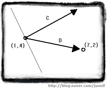 [ 카메라의 시야 ]
 먼저 위의 그림과 같이 카메라의 위치에서 물체의 위치를 가리키는 벡터를 구해야 합니다. 이 벡터를 D = [(7-1) (2-4)] = [ 6 -2 ] 라고 합니다. 이제 벡터 C 와 벡터 D를 내적합니다.
C●D = 5(6) + 3(-2) = 30 - 6 = 24
두 내적의 결과가 양수이므로 두 벡터 사이의 각 θ 는 90˚ 보다 작음을 알 수 있습니다. 카메라의 시야가 90˚이므로 이 물체는 카메라의 시야에 들어옴을 알 수 있습니다.
간단한 계산만으로 두 벡터 사이의 각이 90˚ 에 대하여 큰지 작은지, 혹은 직교하는 지를 알 수 있었습니다. 만일 두 벡터 사이의 정확한 각을 구할 때에도 내적을 통해 알 수 있습니다.
===============================================================
| 두 벡터 사이의 각
| 임의의 두 벡터 A, B 사이의 각을 θ 라 하면,
| A●B = ||A|| ||B|| cos θ
===============================================================
예제를 볼께요.
캐릭터가 벡터 C = [5 2 -3 ]가 가리키는 방향으로 이동중이었습니다. 그런데 플레이어가 새로운 목적지를 설정해 주어서 벡터 D = [8 1 -4 ]가 가리키는 방향으로 이동하게 되었습니다. 이 캐릭터는 얼마의 각을 꺽어야 새로운 경로로 이동 할 수 있을까요?
위의 공식에 대입하려면 먼저 두 벡터의 내적을 구해야 합니다.
C●D = 5(8) + 2(1) -3(-4) = 40 + 2 + 12 = 54
이제 두 벡터의 크기를 각각 구해줍니다.
||C|| = √5² + 2² + (-3)² = √25 + 4 + 9 = √38
||D|| = √8² +1² + (-4)² = √64 + 1 + 16 = √81
이제 각각의 결과를 공식에 대입합니다.
C●D = ||C|| ||D|| cos θ
54 = (√38)(√81) cos θ
54 / (√38)(√81) = cos θ
54 / ( 6.16 * 9 ) = 54 / 55.44 = cos θ
θ = 13.08˚ <---근사값입니다.
따라서 이 캐릭터는 13.08˚ 꺽어서 움직이면 됩니다.
6. 벡터의 외적
내적은 벡터를 곱하는 방법에 해당합니다. 이번에는 외적을 다뤄볼 차례 입니다. 내적과 외적의 가장 큰 차이점이라면 결과값의 형태이겠네요. 내적은 결과값이 스칼라이고 외적의 결과는 벡터입니다.
============================================================
| 외 적
| 임의의 두 벡터 A = [a1 a2 a3], B = [b1 b2 b3]에 대하여,
| A x B = [(a2b3 - a3b2) (a3b1 - a1b3) (a1b2 - a2b1)]
============================================================
예제를 하나 볼께요
두 벡터 A = [ 5 -6 0 ], B = [1 2 3 ]의 외적을 구하세요.
외적의 결과는 또 다른 벡터가 나오므로, 위의 공식을 사용하여 각 성분을 계산하면 됩니다.
A x B = [(a2b3 - a3b2) (a3b1 - a1b3) (a1b2 - a2b1)]
= [(-6(3) - 0(2)) (0(1) - 5(3)) (5(2) - -6(1)) ]
= [ (-18-0) (0-15) (10+6) ]
= [-18 -15 16 ]
외적의 가장 중요한 성질은 바로 외적의 결과로 만들어진 벡터가 원래 두 벡터와 모두 직교하는 벡터라는 것입니다. 이러한 이유 때문에 외적은 3차원 벡터에 대해서만 정의 됩니다.
================================================================
| 직교 벡터
| A x B 는 두 벡터 A, B 에 모두 수직
================================================================
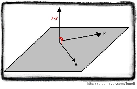 [ 직교 벡터 ]
벡터 A 와 B 를 포함하는 평면에는 수직인 두개의 방향이 있습니다. 바로 위쪽과 아래쪽이죠. 외적의 결과 주어지는 벡터를 결정하는데 오른손 법칙을 쓸 수 있습니다. 손가락을 벡터 A와 B가 교차하는 부분에 두고 손가락을 벡터 A와 같은 방향으로 둡니다. 그런 후에 손가락이 벡터 B를 향하도록 구부리면, 이때 엄지가 향하는 방향이 AxB 의 방향입니다. 반대로 A와 B의 순서를 바꾸어 시도해보면 BxA는 방향이 정반대라는 것을 알 수 있습니다. 그래서 외적은 교환법칙이 성립하지 않습니다.
=====================================================================
| 외적은 교환법칙이 성립하지 않음
| A x B ≠ B x A
| 단, 임의의 3차원 벡터 A , B에 대해서 A x B = -(B x A)
=====================================================================
외적은 결과가 원래의 두 벡터와 수직인 세번째 벡터를 만든다는 독특한 성질 덕뿐에 표면 법선(surface normal)을 계산하는데 사용할 수 있습니다. 임의의 두 3차원 벡터는 하나의 면을 정의합니다. 표면 법선은 주어진 면에 수직인 길이가 1인 벡터를 말합니다.
============================================================
| 표면 법선
| 임의의 두 3차원 벡터 A, B에 대하여,
| 표면 법선 = (A x^ B) = AxB / ||AxB||
=============================================================
**위의 공식에서 x^ 또한 위의 벡터의 부호처럼 ^ 이 x 위에 모자처럼 씌어져야 합니다
역시 예제를 살펴보면 실력을 다져 볼까요?
두 벡터 A = [5 -2 0 ], B = [1 2 3 ]으로 정의되는 면이 있을때, 이 면과 충돌한 물체의 운동을 결정하는데 사용할 수 있도록 표면 법선을 구하십시오.
외적의 결과는 주어진 두 벡터와 직교하는 새로운 벡터이죠? 먼저 외적을 합니다.
A x B = [ (a2b3 - a3b2) (a3b1 - a1b3) (a1b2 - a2b1) ]
= [ (-2(3) - 0(2)) (0(1) - 5(3)) (5(2) - -2(1)) ]
= [ (-6 - 0) (0 - 15) (10 + 2) ]
= [ -6 -15 12 ]
외적을 구했으니 이제 외적의 크기를 구합니다.
||A x B|| = √(-6)² + (-15)² + (12)²
= √36 + 225 + 144
= √405
= 20.125
이제 공식에 대입하면 됩니다.
[ -6/20.125 -15/20.125 12/20.125 ] = [0.298 0.745 0.596 ]
이미 위에서 두 벡터 사이의 각을 내적을 사용하여 구하는 법을 배웠습니다. 각을 구하는 데에는 내적이 더 빠릅니다만 이미 외적의 값을 알고 있다면 외적을 사용하여 각을 구하는 법을 사용하는것이 좋습니다.
=========================================================================
| 두 벡터 사이의 각(외적)
| 임의의 두 3차원 벡터 A, B에 대하여
| ||AxB|| = ||A|| ||B|| sin θ
=========================================================================
자 예제 나갑니다. 단 이번에는 풀이가 없고 답만 알려드릴께요. 한번 직접 풀어보시고 답이랑 맞는지 맞춰보세요 ㅋㅋㅋ
<문제> 두 벡터 A = [5 -2 0], B = [1 2 3] 사이의 각을 구하세요.
<답> 약 87.2˚
////////////////////////////////////////////////////////////////////////////////////////////////
//////////////////////////////////////////////////////////////////
//////
에고 에고 평상시보다 양이 배는 많은것 같네 ㅠㅠ 갈수록 올리는 속도가 느려지네 -.-a
아래 설명의 출처 Direct 3D 기초 수학 #1 벡터 |작성자 야누스
Direct 3D 기초 수학 #1 벡터
* 벡터 : 크기와 방향을 가지는 물리량
* 포인트 (점,Vertex): 한점또는 위치만을 가진다
* 스칼라(Scalar : 크기 . 길이등 한가지만을 표현할때 사용
* 단위벡터 : 크기가 1인 벡터 표기는 ||V|| 와 같이한다.
- 단위벡터는 광선의 방향, 편명의 법선방향 , 카메라의 방향등 방향을 나타낼때
사용된다 크기가 1이 아닌 벡터를 단위벡터로 만들어주는 과정을 정규화(Normalize)
라고 하며 벡터를 자신의 크기로 나눠줌으로 얻을수 있다
벡터의크기 : 벡터 U의 크기 ||U|| = sqrt(Ux^,Uy^,Uz^);
단위벡터 : U / ||U|| ;
*내적의 정의 : 내적의 곱의 결과값은 스칼라이므로 스칼라곱(scalar product)이라고 한다 .
두개 의 벡터 A , B 의 내적을 구해보자
∮(각 세타이다)
내적구하는공식
A * B = = AxBx + AyBy + AzBz ;
두벡터간의 사이갓을 구하는공식
A * B = || A || * || B || cos∮ = cos∮ = A * B / || A || || B || =
∮ = 1/cos(A * B / || A || || B ||) ;
두벡터의 사잇각의 관계
A * B = 0 이면 A ⊥ B 이다
A * B > 0 이면 사잇각은 90보다 작다
A * B < 0 이면 사잇각은 90 보다 크다
A 투영 B ( B에 평행한 분해 벡터) = ((내적) / (B의 Length) * (B의 Length)) * B벡터 ;
A 수직 B ( B에 수직한 분해 벡터 ) = A - ((내적) / (B의 Length) * (B의 Length)) * B벡터 ;
외적의 정의 : 원전에 접선된 두개의 접선벡터에 수직한 벡터를 결과로 갖는 값 .
법선벡터를 구할때 사용한다 .
한평면의 세점 A , B , C 에 대하여 A(Ax,Ay,Az),B(Bx,By,Bz) ,C(Cx,Cy,Cz)에 대하여
점 A를 기준으로 점 B 와 C 에 대한 벡터를 각각 U , V 라 할때 수식을 통하여 벡터를 구할수잇다
U = B(Bx,By,Bz) - A(Ax,Ay,Az) = [Bx -Ax , By - Ay , Bz - Az];
V = C(Cx,Cy,Cz) - A(Ax,Ay,Az) = [Cx - Ax , Cy - Ay, Cz - Az];
두벡터간의 법선 벡터를 구하면 외적을 구할수 있다
외적구하는 공식
x = Uy * Vz - Uz * Vy;
y = Uz * Vx - Ux * Vz;
Z = Ux * Vy - Uy * Vx; 새로운 벡터 E(Ex,Ey,Ez) 두벡터 U,V에 직각인 법선벡터이다 .
D3DX에서 사용되는 함수 이다 , D3DXVECTOR3 클래스는 라이브러리에서 지원되는 클래스이다
크기 : float D3DXVec3Length(D3DXVECTOR* pV);
설명 : 반환값은 스칼라이고 전달인자는 벡터의 &(포인터)이다.
ex) float magnitude = D3DXVec3Length(&V);
단위벡터(Normalize : 정규화) :
D3DXVECTOR3* D3DVec3Normalize(D3DXVECTOR3* pOut,D3DXVECTOR3* pV);
설명 : 반환값은 벡터의 포인터 형태이고 전달인자는 정규화가 끝난 값을 보관할 벡터의 포인터형과 정규화할 벡터의 포인터형태이다
ex) D3DXVECTOR3 U = D3DXVec3Normalize(&pOut,&pV);
내적(Dot product) float D3DXVec3Dot(D3DVECTOR3* pV1 , D3DVECTOR3* pV2);
설명 : 반환값은 스칼라이며 인자는 왼쪽의 피연산벡터의 포인터 , 오른쪽 피연산벡터의 포인터이다
ex)float result = D3DXVec3Dot(&pV1, &pV2);
외적(Corss product) :
D3DVECTOR3* D3DXVec3Cross(D3DXVECTOR3* pOut,D3DVECTOR3* pV1,D3DVECTOR3* pV2);
설명 : 반환값은 연산이 완료된 벡터의 포인터이고 인자는 리턴하기전 결과를 저장할 벡터의 포인터, 왼쪽 피연산벡터의 포인터 , 오른쪽 피연산벡터의 포인터);
ex D3DVECTOR3 Cross = D3DXVec3Cross(&pOut,&pv1 , &pv2);
기억하면 좋을 사항
외적은 교환법칙이 성립되지않는다 , U * V = - (V * B) 이다
벡터의 곱이 스칼라 이면 내적이고 벡터의 곱이 벡터이면 외적이다